
파이썬 분석 실무, 유저 Funnel 분석 - (6) EDA, 일별 주요 통계
03 Nov 2018 | python EDA datetimepython 분석 실무, 유저 funnel 분석 따라 공부하기
- 데이터 불러오기
- 날짜 데이터 다루기
- 결측치 처리
- 예측 모델을 통한 결측치 처리
- 데이터 전처리
- EDA, 일별 주요 통계
EDA(탐색적 데이터 분석, Exploratory Data Analysis)
데이터 전처리를 마쳤다면, 데이터를 둘러보며 어떤 것이 의미있는 정보인지 확인해야 한다. 기본적으로 날짜데이터가 있는 경우는 날짜의 연도/월/일/요일 등 어떤 타입의 날짜 데이터와 연관성이 있는지 알아본다. 유저의 로그를 가지고 분석하는 경우 특정 행동끼리의 상관성도 살펴볼 수 있다.
여기에서는 아래와 같이 EDA를 진행한다.
- 일별 주요 통계 <- 이 글에서는 여기
- 변수별 특성
- 구간별 전환율(Funnel Analysis)
- 클러스터링
- 클러스터별 전환율 차이 파악
기본 트렌드 체크
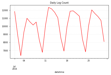
- 일별 로그 카운트 : 일별로 해당 액션이 일어난 수
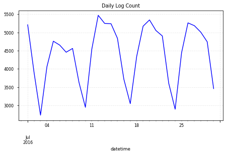
- 일별 세션 카운트 : 일별로 해당 액션을 한 유닉크 유저수
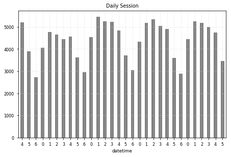
- 요일별 세션 카운트 : 요일별로 해당 액션을 한 유니크 유저수 트렌드
# daily log size

df.groupby('datetime').size().plot(c='r');

plt.title("Daily Log Count")
plt.grid(color='lightgrey', alpha=0.5, linestyle='--')
plt.tight_layout()
# daily session counts => Active index

df.groupby('datetime')['sessionid'].nunique().plot(c='b');

plt.title("Daily Log Count")
plt.grid(color='lightgrey', alpha=0.5, linestyle='--')
plt.tight_layout()
## daily session count (weekofday)
# 0: Monday, 6: Sunday

s = df.groupby("datetime")['sessionid'].nunique()
s.index = s.index.dayofweek # datetime 요일로 변환

s.plot(color='grey', kind='bar', rot=0);

plt.title("Daily Session")
plt.grid(color='lightgrey', alpha=0.5, linestyle='--')
plt.tight_layout()
 0: Monday, 6: Sunday
Note.
- 앱 로그에 sessionality 존재
- 로그 수와 세션수 트렌드가 유사
- 주말에 사용성이 매우 감소하고 주중 초반이 높은 편
- 문서앱이라는 특성상, 직장인 혹은 학생이 주로 사용할 것으로 가정하면 당연한 결과
해당 서비스에 맞는 일별 트렌드 확인
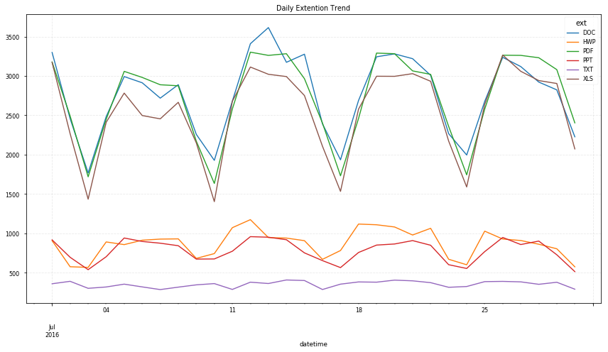
- 일별, 확장자별 로그수
- 일별, 위치별 로그수
- 일별, 액션별 로그수
- 일별, 화면 스크린별 유니크 유저수
# daily trend by extention
df.groupby(['datetime', 'ext']).size().unstack().dropna(axis=1).plot(figsize=(12,7));

plt.title("Daily Extention Trend")
plt.grid(color = 'lightgrey', alpha=0.5, linestyle='--') # alpha는 투명도
plt.tight_layout()
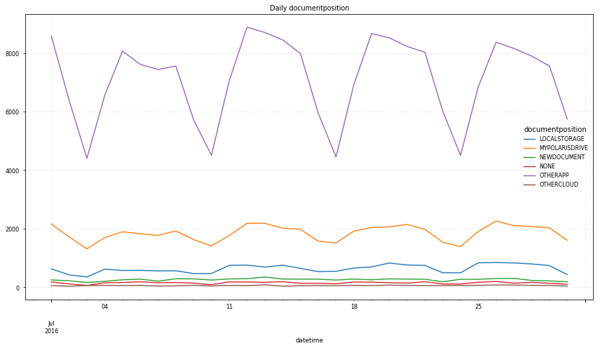
# daily trend by doc position
df.groupby(['datetime', 'documentposition']).size().unstack().dropna(axis=1).plot(figsize=(12, 7));

plt.title("Daily documentposition")
plt.grid(color='lightgrey', alpha=0.5, linestyle='--')
plt.tight_layout()
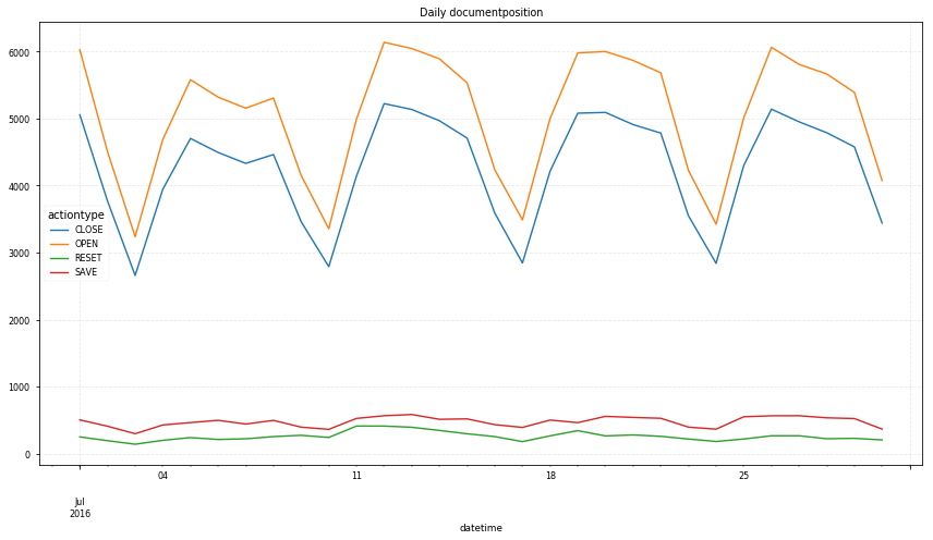
# daily trend by action type
df.groupby(['datetime', 'actiontype']).size().unstack().dropna(axis=1).plot(figsize=(12, 7));

plt.title("Daily documentposition")
plt.grid(color='lightgrey', alpha=0.5, linestyle='--')
plt.tight_layout()
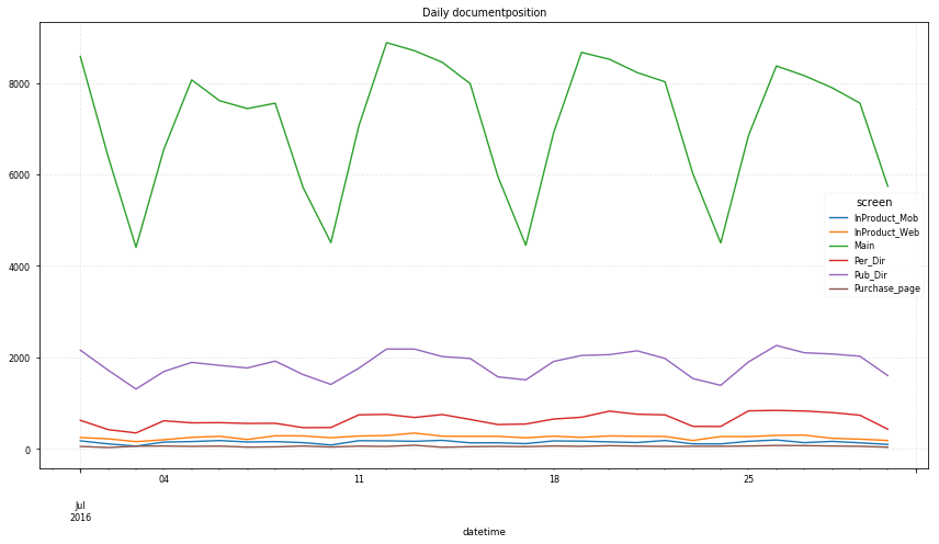
# daily trend by screen name
df.groupby(['datetime', 'screen']).size().unstack().dropna(axis=1).plot(figsize=(12, 7));

plt.title("Daily documentposition")
plt.grid(color='lightgrey', alpha=0.5, linestyle='--')
plt.tight_layout()
#heat map
screens = df.groupby(['datetime', 'screen'])['sessionid'].nunique().unstack().fillna(0).astype(int)
# cols order change
screens = screens[screens.mean().sort_values(ascending=False).index]

plt.subplots(figsize=(17,8))

sns.heatmap(screens, annot=True, fmt='d', annot_kws={'size':12}, cmap='Blues');

plt.title("screen count daily")
plt.tight_layout()
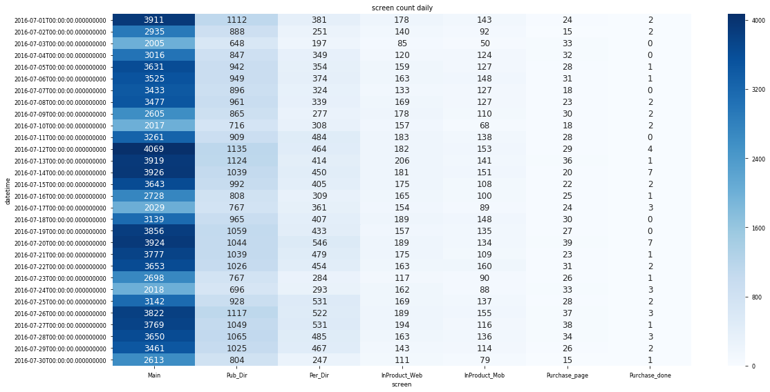
Note.
- doc, pdf, xls 순으로 주로 사용
- 주요 문서 이용 위치는 otherapp
- Main -> 구매완료(purchase_done) 까지 과정에서 대부분 이탈
이 글에서 사용한 Pandas 함수 정리
groupby()
특정 항목을 기준으로 갯수, 평균 등의 수치를 보고 싶을 때, 유용한 함수이다. 여기에서는 날짜별 로그수, 세션수 등을 봤다. plot()과 함께 쓰면, 따로 해당 데이터를 값으로 저장하지 않고 바로 경향성을 그래프로 확인할 수 있다.
.groupby([col1, col2]).apply(): 앞에 있는 칼럼으로 먼저 묶인다..groupby([col1, col2])['col3'].apply(): 구분은 col1, col2이지만, 값은 col3에 대한 걸 보고 싶을 때- apply 부분에 사용할 수 있는 함수들
df.groupby('A').sum()- 해당 내용 항목별로 카테고리 묶음,숫자데이터 다른 칼럼 값끼리 더함
df.groupby('A').size()- 해당 내용 항목별로 카테고리 묶음, 그 사이즈 확인
- Series의
.value_counts()와 비슷
df.groupby('A')['B'].nunique()- ‘A’ 내용 항목별로 카테고리 묶고, 거기의 ‘B’ 유니크한 값 숫자 확인
-
df.groupby.reset_index(): 구분으로 사용한 칼럼값을 index로 쓰고 싶지 않을때, 구분으로 묶은 것을 값으로 넣어서 출력함df.groupby(['datetime', 'ext']).size().reset_index().head() # datetime ext 0 # 0 2016-07-01 DOC 3298 # 1 2016-07-01 HWP 908 # 2 2016-07-01 PDF 3177 # 3 2016-07-01 PPT 918 # 4 2016-07-01 SHEET 2 df.groupby.unstack(level=0): povot, stack, groupby 함수에 의해 기준칼럼이 값별로 row에 있는 것을 col로 옮겨서 출력해줌- Q. prefix, sufix 넣는 방법은 없나..?
  df.groupby(['datetime', 'screen'])['sessionid'].nunique().unstack().head()

  # screen	InProduct_Mob	InProduct_Web	Main	Per_Dir	Pub_Dir	Purchase_done	Purchase_page
  # datetime
  # 2016-07-01	143.0	178.0	3911.0	381.0	1112.0	2.0	24.0
  # 2016-07-02	92.0	140.0	2935.0	251.0	888.0	2.0	15.0
  # 2016-07-03	50.0	85.0	2005.0	197.0	648.0	NaN	33.0
  # 2016-07-04	124.0	120.0	3016.0	349.0	847.0	NaN	32.0
  # 2016-07-05	127.0	159.0	3631.0	354.0	942.0	1.0	28.0
plot()
pandas.DataFrame.plot에서 이번에 썼던 것만 봐보자.
.gird().title()tight_layout()- X(index),Y(column)으로 plotting
# groupby 이후에 unstack() 사용한 이유, X,Y 잡아주기

df.groupby(['datetime', 'ext']).size().unstack().dropna(axis=1).plot(figsize=(12,7));
sns.heatmap()
seaborn.heatmap를 한번 봐보자.
- parameters
annot: bool or rectangular dataset, optionalIf True, write the data value in each cell. If an array-like with the same shape as data, then use this to annotate the heatmap instead of the raw data.
fmt: string, optionalsns.heatmap(screens, annot=True, fmt='d', annot_kws={'size':12}, cmap='Blues');String formatting code to use when adding annotations.
annot_kws: dict of key, value mappings, optional, 값 텍스트 부분 설정Keyword arguments for ax.text when annot is True.
Numbers formatting with format() 1
포맷 코드로 숫자와 글 이용하기
-
For positional arguments(순서 위치로 포맷 이용)
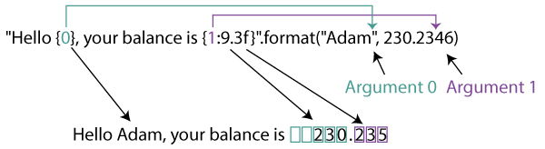
-
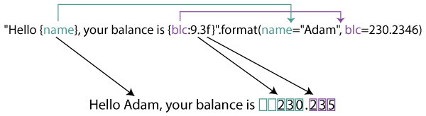
For keyword arguments(값을 지정해 포맷 이용)
Numbers formatting with
| Type | Meaning |
|---|---|
| d | Decimal integer |
| c | Corresponding Unicode character |
| b | Binary format |
| o | Octal format |
| x | Hexadecimal format (lower case) |
| X | Hexadecimal format (upper case) |
| n | Same as ‘d’. Except it uses current locale setting for number separator |
| e | Exponential notation. (lowercase e) |
| E | Exponential notation (uppercase E) |
| f | Displays fixed point number (Default: 6) |
| F | Same as ‘f’. Except displays ‘inf’ as ‘INF’ and ‘nan’ as ‘NAN’ |
| g | General format. Rounds number to p significant digits. (Default precision: 6) |
| G | Same as ‘g’. Except switches to ‘E’ if the number is large. |
| % | Percentage. Multiples by 100 and puts % at the end. |